Helen believes that the random variable C, representing cloud cover from the large data set, can be modelled by a discrete uniform distribution.

(a) Write down the probability distribution for C.


(b) Using this model, find the probability that cloud cover is less than 50%


Helen used all the data from the large data set for Hurn in 2015 and found that the proportion of days with cloud cover of less than 50% was 0.315

(c) Comment on the suitability of Helen’s model in the light of this information.


(d) Suggest an appropriate refinement to Helen’s model.

Tessa owns a small clothes shop in a seaside town. She records the weekly sales figures, £ w, and the average weekly temperature, t °C, for 8 weeks during the summer.

The product moment correlation coefficient for these data is −0.915

(a) Stating your hypotheses clearly and using a 5% level of significance, test whether or not the correlation between sales figures and average weekly temperature is negative.


(b) Suggest a possible reason for this correlation.


Tessa suggests that a linear regression model could be used to model these data.

(c) State, giving a reason, whether or not the correlation coefficient is consistent with Tessa’s suggestion.


(d) State, giving a reason, which variable would be the explanatory variable.


Tessa calculated the linear regression equation as \({w = 10755 - 171t}\)

(e) Give an interpretation of the gradient of this regression equation.

In an experiment a group of children each repeatedly throw a dart at a target.
For each child, the random variable H represents the number of times the dart hits the target in the first 10 throws.

Peta models H as B(10, 0.1)

(a) State two assumptions Peta needs to make to use her model.


(b) Using Peta’s model, find \({P(H⩾4)}\)


For each child the random variable F represents the number of the throw on which the dart first hits the target.

Using Peta’s assumptions about this experiment,

(c) find \(P(F=5)\)


Thomas assumes that in this experiment no child will need more than 10 throws for the dart to hit the target for the first time. He models \({P(F=n)}\) as:
\[P(F=n)=0.01+(n−1)×α\]
where α is a constant.

(d) Find the value of α


(e) Using Thomas’ model, find \({P(F=5)}\)


(f) Explain how Peta’s and Thomas’ models differ in describing the probability that a dart hits the target in this experiment.

Charlie is studying the time it takes members of his company to travel to the office. He stands by the door to the office from 0840 to 0850 one morning and asks workers, as they arrive, how long their journey was.

(a) State the sampling method Charlie used.


(b) State and briefly describe an alternative method of non-random sampling Charlie could have used to obtain a sample of 40 workers.


Taruni decided to ask every member of the company the time, x minutes, it takes them to travel to the office.

(c) State the data selection process Taruni used.


Taruni’s results are summarised by the box plot and summary statistics below.



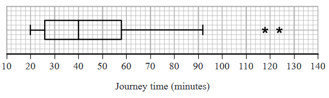
\[n = 95 \quad \sum{x} = 4133 \quad \sum{x^2} = 202294 \]

(d) Write down the interquartile range for these data.


(e) Calculate the mean and the standard deviation for these data.


(f) State, giving a reason, whether you would recommend using the mean and standard deviation or the median and interquartile range to describe these data.


Rana and David both work for the company and have both moved house since Taruni collected her data.

Rana’s journey to work has changed from 75 minutes to 35 minutes and David’s journey to work has changed from 60 minutes to 33 minutes.

Taruni drew her box plot again and only had to change two values.

(g) Explain which two values Taruni must have changed and whether each of these values has increased or decreased.

The lifetime, L hours, of a battery has a normal distribution with mean 18 hours and standard deviation 4 hours.

Alice’s calculator requires 4 batteries and will stop working when any one battery reaches the end of its lifetime.

(a) Find the probability that a randomly selected battery will last for longer than 16hours.


At the start of her exams Alice put 4 new batteries in her calculator.
She has used her calculator for 16 hours, but has another 4 hours of exams to sit.

(b) Find the probability that her calculator will not stop working for Alice’s remaining exams.


Alice only has 2 new batteries so, after the first 16 hours of her exams, although her calculator is still working, she randomly selects 2 of the batteries from her calculator and replaces these with the 2 new batteries.

(c) Show that the probability that her calculator will not stop working for the remainder of her exams is 0.199 to 3 significant figures.


After her exams, Alice believed that the lifetime of the batteries was more than 18 hours. She took a random sample of 20 of these batteries and found that their mean lifetime was 19.2 hours.

(d) Stating your hypotheses clearly and using a 5% level of significance, test Alice’s belief.